Detecting Data Drift

In this post we will cover some of the techniques used to identify any data drift that might be going on.

Say you’ve deployed a model into production and you notice that the performance is degrading. There are a few possible causes behind the performance degradation:

There are errors in the model input data itself:
- The input data maybe erroneous due to problems with the data source. Front end issues mean that the data being written into the database is incorrect
- There may be errors in the feature engineering calculations. The data at the source is correct but there is an error in the pipeline or during feature engineering which means that the data input into the model for a particular feature is incorrect
These issues usually require further human investigation and can be resolved through code reviews, debugging, etc.
When there is a real change in the data due to external factors. This is data drift and in Part 1 of this series we learned about the different types of data drift (covariate shift, prior probability shift & concept shift) and some examples.

Let’s say after some checks, you suspect that the model performance degradation is indeed due to data drift. So how can we verify this and identify where in our data the data drift is occuring?

There are three main techniques to measure drift:

Statistical: This approach uses various statistical metrics on your datasets to come to a conclusion about whether the distribution of the training data is different from the production data distribution. We already have the data and so it usually involves running the same calculation each time and maybe plotting the results for easier analysis.
Model Based: This approach involves training a classification model to determine whether certain data points are similar to another set of data points. If the model has a hard time differentiating between the data, then there isn’t any significant data drift. If the model is able to correctly separate the data groups, then there likely is some data drift.
Adaptive Windowing (ADWIN): This approach is used with streaming data, where there is a large amount of infinite data flowing in and it is infeasible to store it all. At the same time, the data can change very quickly.

1. Statistical Approach

Many of these approaches compare distributions. A comparison requires a reference distribution which is the fixed data distribution that we compare the production data distribution to. For example, this could be the first month of the training data, or the entire training dataset. It depends on the context and the timeframe in which you are trying to detect drift. But obviously, the reference distribution should contain enough samples to represent the training dataset.

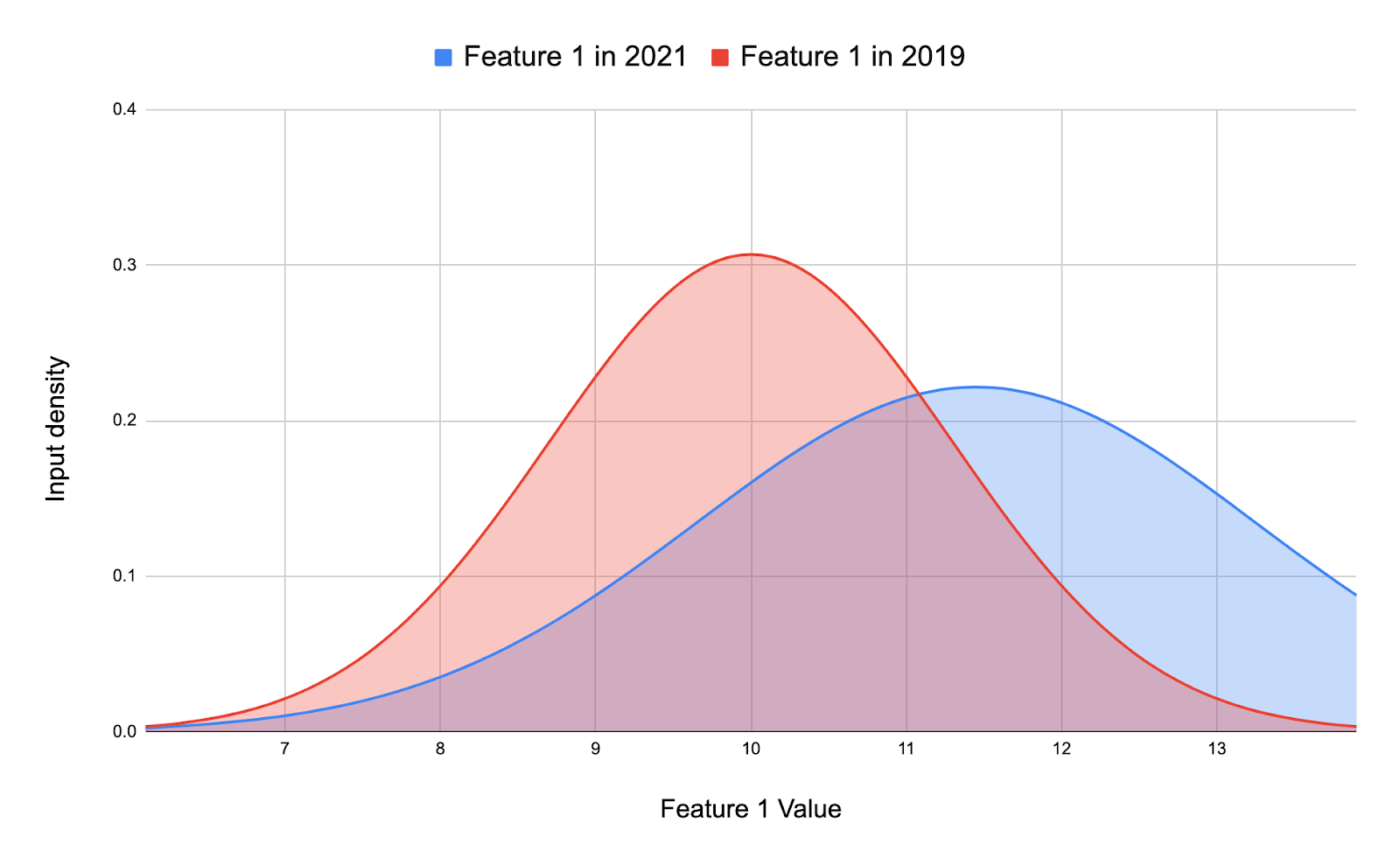
For simplicity, let’s say we have a classification model with 10 features. Let’s say Feature A and Feature B are some of the top contributing features of the model. For this post let’s look at how we can go about trying to see whether features A and B have data drift happening. For the following measures we will be comparing the training dataset to an out-of-time labelled data to which we know the ground truth. So say the model has been trained on data from 2019, and the performance has been slowly degrading through 2020. So we will look for data drift in Feature A and B between 2019 and 2020. In reality, we can repeat the following for the other features as well (at least the top features).

NOTE: Since we want to observe data drift over time, we want to aggregate or divide the data by time which can be monthly, weekly, etc depending on your data and monitoring frequency. In this example we will aggregate data on a monthly basis.

Below I will explain some of the different statistical methods used to detect drift. To see a full example with code using a real dataset please refer my blog post here

Mean

One of the first and simplest measures we can look at is the means for our features. If the mean gradually shifts in a particular direction over the months, then there probably is data drift happening. The mean isn’t the most sound check of checking for drift but is a good starting point.

mean_trends

Statistical Distance Measures

There are a number of different statistical distance measures that can help quantify the change between distributions. Different distance checks are useful in different situations.

Population Stability Index (PSI)

PSI is often used in the finance industry and is a good metric for both numeric and categorical when the distributions are fairly stable. As the name suggests it helps measure the population stability between two population samples.

Equation: PSI = (Pa — Pb)ln(Pa/Pb)

The ln(Pa/Pb) term implies that a large change in a bin that represents a small percentage of a distribution will have a larger impact on PSI than a large change in a bin with a large percentage of the distribution.

It should be noted that the population stability index simply indicates changes in the population of loan applicants. However, this may or may not result in deterioration in performance. So if you do notice a performance degradation, you could use PSI to confirm that the population distributions have indeed changed. PSI checks can be added to your monitoring plan too.

Kullback-Leibler (KL) divergence

KL divergence measures the difference between two probability distributions and is also known as the relative entropy. KL divergence is useful if one distribution has a high variance or small sample size relative to the other distribution.

KL_formula

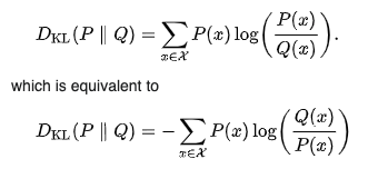
KL divergence is also not symmetric. This means that unlike PSI, the results will vary if the reference and production(compared) distributions being compared are switched. So KL(P || Q) != KL(Q || P). This makes it useful for applications involving Baye’s theorem or when you have a large number of training (reference) samples but only a small set of samples (resulting in more variance) in the comparison distribution.

A KL score can range from 0 to infinity, where a score of 0 means that the two distributions are identical. If the KL formulae are taken to log base 2, the result will be in bits, and if the natural log (base-e) is used, the result will be in “nats”.

Jensen-Shannon (JS) Divergence

The JS divergence is another way to quantify the difference between two probability distributions. It uses the KL divergence that we saw above to calculate a normalized score that is symmetrical. This makes JS divergence score more useful and easier to interpret as it provides scores between 0 (identical distributions) and 1 (maximally different distributions) when using log base 2.

With JS there are no divide-by-zero issues. Divide by zero issues come about when one distribution has values in regions the other does not.

Wasserstein distance metric

The Wasserstein distance, also known as the Earth Mover’s distance, measures the distance between two probability distributions over a given region. The Wasserstein Distance is useful for statistics on non-overlapping numerical distribution moves and higher dimensional spaces, for example images.

Kolmogorov–Smirnov test (K–S test or KS test)

The KS test is is a nonparametric test of the equality of continuous/discontinuous, one-dimensional probability distributions that can be used to compare a sample with a reference probability distribution (one-sample K–S test), or to compare two samples (two-sample K–S test).

2. Model Based

An alternative to the statistical methods explored above is to build a classifier model to try and distinguish between the reference and compared distributions. We can do this using the following steps:

Tag the data from the batch used to build the current production model as 0.
Tag the batch of data that we have received since then as 1.
Develop a model to discriminate between these two labels.
Evaluate the results and adjust the model if necessary.

If the developed model can easily discriminate between the two sets of data, then a covariate shift has occurred and the model will need to be recalibrated. On the other hand, if the model struggles to discriminate between the two sets of data (it’s accuracy is around 0.5 which is as good as a random guess) then a significant data shift has not occurred and we can continue to use the model.